These materials may be used for teaching purposes if the credit is included.
NOTE: Captions in the images are mostly in German.
Any kind of further use requires the renewed approval by the GFZ.

Inner structure of the Earth: The hot core of the Earth consists of a solid inner core (temperatures of up to 5000 °C) and a liquid outer core. The Earth's mantle curves over this (temperature at the core/mantle boundary is over 3000 °C). The Earth's crust, with an average thickness of 40 km, is the thin outer skin of the planet and our habitat. The enormous heat in the Earth's interior is the engine for plate tectonics and, in a broader sense, for almost all dynamic processes of the Earth's body.
![[Translate to English:] GPS measurements | Plate tectonic movement (1994-2016)](/fileadmin/_processed_/9/f/csm_stations_horizontal_with_plates_35070976a9.jpg)
Plate tectonic movement: The large lithospheric plates and their directions of movement based on 23 years (1994 - 2016) GPS measurement

Animation | The break-up of Pangaea: The animation shows the plate tectonic development of the last 230 million years (Müller et al., 2016), reconstructed using GPlates (www.gplates.org). In this plate reconstruction, today's political boundaries and topography are shown for orientation (Amante & Eakins, 2009, illustrations: S. Brune, GFZ). The break-up of Pangaea was initiated about 200 million years ago. Around 150 million years ago, the Atlantic Ocean had already partially opened up and the northern continent of Laurasia was largely separated from the southern continent of Gondwana. India, Antarctica and Australia began to separate from Africa. The South Atlantic had already opened up 100 million years ago. India moved north towards Asia.
References: Amante, C., & Eakins, B. W. (2009). ETOPO1 1 Arc-Minute Global Relief Model: Procedures, Data Sources and Analysis. NOAA Technical Memorandum NESDIS NGDC-24. National Geophysical Data Center, NOAA.(https://doi.org/10.7289/V5C8276M)
Müller, R. D., Seton, M., Zahirovic, S., Williams, S. E., Matthews, K. J., Wright, N. M., et al. (2016). Ocean Basin Evolution and Global-Scale Plate Reorganization Events Since Pangea Breakup. Annual Review of Earth and Planetary Sciences, 44(1), 107-138. (https://doi.org/10.1146/annurev-earth-060115-012211http

Global distribution of earthquakes & volcanoes: The global distribution of volcanoes and earthquakes is closely linked to the plate boundaries. On land, around 1500 volcanoes are considered potentially active. Red triangles = volcanoes, purple dots = earthquakes
 project has produced a world map of earthquake hazard. Shown (in color) is the probability of exceeding classes of horizontal acceleration ...")
World map of earthquake hazard: The GSHAP (Global Seismic Hazard Program) project has produced a world map of earthquake hazard. Shown (in color) is the probability of exceeding classes of horizontal acceleration during earthquakes.
Download
 and shows the seismic hazard as peak ground acceleration (PGA, ms-2) with a 10% probability of exceedance.")
Seismic Hazard Map Europe: The map is part of the Global Seismic Hazard Map (Grünthal et al., 1999) and shows the seismic hazard as peak ground acceleration (PGA, ms-2) with a 10% probability of exceedance in 50 years, which corresponds to a return period of 475 years.

Earthquakes in Europe: The epicenters of the cataloged earthquakes for magnitudes Mw ≥ 6 of the last 1000 years as well as plate boundaries (red) and selected first-order faults (black) are shown. Source GFZ-EMEC (European-Mediterranean Earthquake Catalogue for the last millennium)
. This is creating fault lines on the North Anatolian...")
Risk of earthquakes in Turkey: The small Anatolian plate is shifted westwards between the northward drifting Arabian plate and the Eurasian plate (lateral displacement). This creates tension in the North Anatolian Fault Zone, which results in severe earthquakes. In 1999 alone, two earthquakes with a magnitude of over M = 7.5 caused more than 19,000 deaths in the area of the North Anatolian Fault.

Earthquake sequence Nepal 25.04. and 12.05.2015: On the poster you will find detailed information on the earthquake sequence in Nepal (25.4. and 12.5.2015). Further earthquake posters are available on the pages of Section 2.1 Earthquake and Volcano Physics.


Subduction process and Sumatra tsunami 2004: At the Sunda Trench, the Indo-Australian plate is sliding under the Eurasian plate at a rate of 6 - 8 cm/year. The subduction of the Indian plate under Eurasia caused Sumatra to bend downwards. The stress-induced fracture led to a jerky upward movement of the sea floor. This vertical impulse generated the tsunami.
![[Translate to English:] Animation earthquake sequence Sumatra](/fileadmin/gfz/medien_kommunikation/Schulen/Unterrichtserg%C3%A4nzendes_Material/Abbildungen/GEOFON_GFZ_Animation_Sumatrabeben_2004.gif)
Animation of the earthquake sequence off Sumatra, 26.12.2004
Animation of the distribution and magnitude of earthquakes between 26.12.2004 and 10.01.2005.

Modeling of the tsunami of 26.12.2004 off Sumatra
Complete animation in high resolution

Animation of the earthquake sequence in Japan, 11.03.2011
Animation of the distribution and strength of the foreshocks and aftershocks between March 8 and 16, 2011. The GEOFON Earthquake Information Service of the GFZ registered a total of 1538 aftershocks of the Tohoku earthquake of March 11, 2011 by the end of February 2012, 56 of which were magnitude 6 or greater.

Propagation and wave heights of the tsunami of 11.03.2011: This model calculation shows the strength and propagation of the tsunami that hit Sendai Province and the Fukushima nuclear power plant. Tsunamis travel almost undisturbed through entire oceans.

The world's first remote recording of an earthquake: On April 17, 1889, the young scientist Ernst von Rebeur-Paschwitz succeeded in making the world's first remote recording of an earthquake. On Potsdam's Telegrafenberg, today's headquarters of the German Research Center for Geosciences, he used a pendulum apparatus to record an earthquake that occurred in the Pacific, near Japan.

Subduction of a continental plate: Cross-section through the Earth's crust and upper mantle in the Pamirs. In 2013, GFZ researchers were able to directly observe the subduction of a piece of continental plate under a continental plate for the first time. The Pamir Mountains are located in the northernmost part of the collision zone between India and Eurasia. Both shallow and deep earthquakes occur at the collision zone (shown by white circles). The deep earthquakes are caused by the subduction of the lower Eurasian crust. Black triangles: Location of the seismometer chain.

Soil animal memory (primary school): The memory contains 21 animals and their distinguishing features (body length, number of legs). It can be played as a pure picture memory and as a picture-text memory.

Soil animals identification table (primary school): Many different soil animals live in the upper soil layers. These are sometimes so small that they can only be recognized with a magnifying glass. Important identification and distinguishing features are the body length and the number of legs.
The identification table contains 21 animals and their distinguishing features (body length, number of legs) and a scale in mm. Available in A3 and A4 format. The respective documents should be printed in the original size (actual size in Adobe Acrobat) due to the scale.
Download A4 | Download A3
GFZ-Satelliten: GRACE, Swarm, CHAMP
 is to measure the Earth's gravitational pull and its change over time with unprecedented accuracy. The GRACE satellites also")
GRACE: The main objective of the GRACE mission (Gravity Recovery And Climate Experiment) is to measure the Earth's gravitational field and its change over time with unprecedented accuracy over a period of >5 years. The GRACE satellites also probe the Earth's atmosphere and determine global vertical temperature and water vapor distributions from GPS radio occultation measurements. The model of the Earth's gravity created from CHAMP and GRACE data has become famous as the Potsdam potato. GRACE is used to record climate-related mass displacements (ice, water) in the Earth system, e.g. the change in ice mass in Greenland or the Antarctic or the seasonal variation in continental water storage (Image: Astrium/GFZ).

CHAMP: From mid-2000 to September 2010, the CHAMP (Challenging Minisatellite Project) satellite measured the Earth's gravity and magnetic field and determined global vertical temperature and water vapor distributions from GPS radio occultation measurements. CHAMP was the founding father of an entire generation of satellites and satellite measurement methods. With its high-precision, multifunctional, complementary payload elements (magnetometer, accelerometer, star sensor, GPS receiver, laser retroreflector, ion drift meter), CHAMP was the first to deliver high-precision gravity and magnetic field measurements simultaneously (Image: Astrium/GFZ)

The irregular gravitational field of the Earth - The Potsdam gravity potato: Due to the differences in mass in the Earth's interior, the mass-dependent gravitational field is not the same everywhere. In the image, the irregularities in the Earth's gravitational field are shown as deviations from the rotational ellipsoid with a 15,000-fold exaggeration. A lowering of the sea level south of India is recognizable. In this area, the sea level is around 105 m below the ellipsoid of rotation. The geoid heights above the oceans are colored from dark blue (-105 m) to red (+85 m), green/yellow marks the zero line. The continents are shown in gray for better orientation.

Geoid height: The geoid height N is the deviation of the normal-zero height reference surface from the ellipsoid of rotation. The terrain height H is defined as the height above sea level and represents the real height of the topography above the geoid height. (Fig.: GFZ)

Glacial isostatic adjustment: The melting of large ice masses relieves the lithosphere and causes it to rise. The viscous rock of the upper mantle does not flow as quickly. This creates a local mass deficit.
![[Translate to English:] GRACE/GRACE-FO - Monitoring water shortages in Europe](/fileadmin/_processed_/a/a/csm_Grace_Europakarten_TWS_59fcdceae1.png)
GRACE/GRACE-FO - Water monitoring: Regions in which less water was stored are shown in red; a water surplus is shown in blue. Since 2018, most summers in Europe have been too dry. This led to significant groundwater deficits in many areas. The maps show the regions of Europe in which terrestrial water storage (TWS) shows a deficit in May. The situation in Ukraine is most striking but large parts of Germany have also been affected by drought and water shortages for several years now.

Sea level rise: The figure shows the rise in sea level (after subtraction of the mean annual cycle), broken down into the following components: Meltwater (light blue; from the GRACE/GRACE-FO data), thermal expansion (turquoise) and total rise (dark blue). The GRACE satellite missions represent the only currently known remote sensing concept that provides quantitative information on mass redistributions between continents and oceans. This means that, for the first time, the amount of meltwater contributing to sea level rise can be precisely quantified and visualised as a separate component over time. Meltwater accounts for roughly 50 % of the current total increase. The separation of the various contributions to sea level rise is important for the validation of numerical models, which are employed to forecast future sea level changes.

Swarm: ESA's Swarm satellite mission consists of a constellation of three CHAMP-like satellites orbiting the Earth between 400 and 550 km in three different polar orbits. The main objective of the mission is to observe the Earth's magnetic field and its changes over time with unprecedented accuracy. This data can be used to draw new conclusions about the Earth's interior and near-Earth space. Each satellite will provide high-precision and high-resolution measurements of the magnitude and direction of the Earth's magnetic field. (Image: ESA/AOES Medialab)

Geomagnetic Field Strength at Earth's Surface: The figure shows a map of the magnetic field strength from such a model of the core field, which was calculated from data from the CHAMP and Swarm satellites and from geomagnetic observatories on the ground. An interesting feature of the core field is the so-called South Atlantic Anomaly. This is a large area over South America, the South Atlantic and southern Africa with unusually low field intensity (less than 20,000nT). Find more information here.
![[Translate to English:] Laschamp event](/fileadmin/_processed_/4/1/csm_Laschamp_Titel_3ea6c8d1ec.jpg)
Short-term reversal of the polarity of the Earth's magnetic field during the so-called Laschamp event, around 41,000 years ago: The magnetic field weakened to only 5 % of its current strength and more cosmic radiation reached the Earth. The field lines make the event visible. Temporal fluctuations in the strength and direction of the Earth's magnetic field are signals that can be converted into sound. The orientation of the magnetic field is stored in certain layers of rock that formed at this time. The strength and direction can be analyzed using sediment cores and volcanic rock. In the animation, blue areas show where field lines enter the Earth at the magnetic poles, red areas where they exit. There have even been times with more than two poles. The Earth's magnetic field is constantly changing in space and time. Because it originates in the Earth's liquid outer core, we also learn something about the dynamics of the Earth's interior from the field analysis.
Download: Animation (with sound)
GFZ | Magnetic field reconstruction: Sanja Panovska, Animation: Maximilian Schanner (+UP), Guram Kervalishvili DTU Space | Sound: The Danish sound artist Klaus Nielsen mixed recordings of natural sounds such as creaking wood & falling stones to create familiar and unfamiliar sounds.
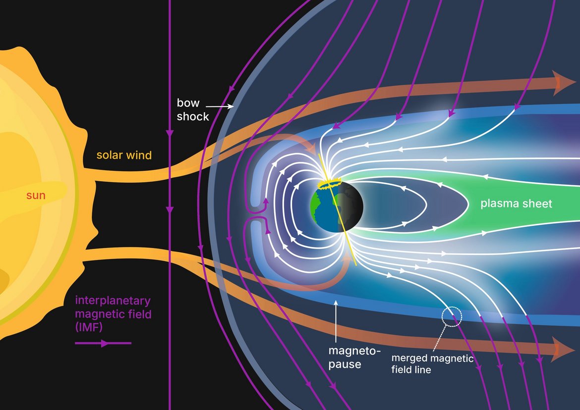
Formation of Auroras: Fast, charged particles from the sun‘s atmosphere collide with the magnetopause, the outer boundary of the magnetosphere. In the process, the solar wind deforms the Earth‘s magnetic field. On the side facing the sun, the solar wind compresses the Earth‘s magnetic field and on the side facing away from the sun, it pulls it apart to form a very long tail. The bow shock forms an arc-shaped front in front of the magnetopause, where the incoming solar wind particles are slowed down from supersonic to subsonic speed. (Note: The relative sizes of the Earth and the sun and the distances between the two bodies are not drawn to scale).
 from the Topex, Jason-1 and Jason-2 missions in mm/year (with GIA correction). The averaged global trend for this period is...")
Change in mean sea level: Sea level trend derived from radar altimeter data (1993 to 2018) from the Topex, Jason-1 and Jason-2 missions in mm/year (with GIA correction). Since the start of global measurements by satellite (1993), global sea level has risen by around 10 centimeters. The average global trend since 2006 is 3.7 (+/-0.6) millimeters per year. However, the rise is not uniform. A rise in the western Central Pacific, for example, contrasts with a fall in sea level on the American west coasts and in the South Pacific.

Global CO2 Cycle: The geological cycle of carbon dioxide. Rock weathering chemically binds the CO2 that is constantly escaping from volcanoes. It reaches the oceans via rivers, where it is bound long-term in calcareous deposits such as coral reefs or foraminifera muds. A lot of CO2 is also disposed of via photosynthesis in sediments that are rich in organic material.

Global beryllium cycle: The mass 9 isotope of the rare element beryllium can be used to determine the amount of sediment that enters the oceans via rivers. The very rare isotope beryllium-10, on the other hand, is produced in the atmosphere by cosmic radiation in constant quantities and enters the oceans via precipitation. If the isotope ratio of 10Be to 9Be fluctuates, this is only due to changes in the input of 9Be from erosion into the sediment. As measurements show, the ratio of the two isotopes to each other in the iron-manganese crusts of all oceans has hardly changed in the last ten million years.
 or in the rock (\"in situ\") against the background of the Forno glacier, Switzerland (Photo: F.von Blanckenburg, GFZ)")
Beryllium nuclide formation: Cosmic rays and production of the isotope beryllium-10 in the atmosphere ("meteoric") or in the rock ("in situ") against the background of the Forno glacier, Switzerland (Photo: F. von Blanckenburg, GFZ).
. Local/regional changes can be measured with high-pre")
The water cycle: Water is mass and therefore exerts gravitational force. Changes in the global water balance can therefore be recorded using satellite measurements (GRACE, GOCE). Local/regional changes can be measured with high-precision superconducting gravimeters and thus provide information about changes in the groundwater balance.

Hydrothermal geothermal drilling: Classic doublet drilling for the use of deep geothermal energy. Hot deep water is pumped out of the Earth with the production well. After the heat has been utilized, the cold water is pumped back underground. (Image: GFZ)

Heating with geothermal energy: How does geothermal energy work? How can you heat houses and apartments in a climate-friendly way with warm water from deep underground? Geothermal energy is renewable, climate-friendly and also available in Germany. It uses the heat beneath the Earth's surface to heat houses or entire settlements. This involves drilling into layers of rock and pumping water upwards. In order to use geothermal energy efficiently, the rocks must be sufficiently permeable. This is because the water is stored in their pores - like in a sponge. Preliminary explorations help to find out where it is worth drilling.